Time Series Analysis with Pandas

Pandas is the operating system in time series projects. It has powerful data manipulation and analysis libraries. Several built-in functions in pandas give you the stage to perform various aggregate calculations on your DataFrame. With Pandas, tasks like resampling, shifting, and rolling window operations become more efficient.

Before starting, some newbies like me in data science might wish to know what time series data is. Time series data is a sequence of observations recorded over regular time intervals. It consists of data points ordered chronologically, allowing analysis of trends, patterns, and behaviours over time. Some examples of time series data include stock prices, weather measurements, and monthly sales figures.

Enough of abstractions! Let’s analyze a monthly sales figure dataset to demonstrate basic operations in analyzing time series with pandas. Remember, Pandas alone cannot be used for a whole data analysis. So we shall use other data science libraries like Numpy, Matplotlib, and Seaborn with Pandas.

Loading Time Series Data into Pandas DataFrame

---

Download the sale figure dataset here.

---

To load time series data into a Pandas DataFrame, you can use the pd.read_csv() function for CSV files, pd.read_excel(), pd.read_sql(), and pd.read_json() for Excel, SQL, and JSON files. It all depends on your dataset format.

Our sale figure dataset is a CSV file. Thus, we use the .read_csv() method to read it.

import pandas as pd
# Load the downloaded dataset, where 'path/to/file/train.csv' is the path # location of the  train.csv file on your local machine.

data = pd.read_csv('path/to/file/train.csv', delimiter = ',') 

# Display the first five rows of the dataset
data.head()

Output:

# check the datatype of each column in the dataset
data.dtypes

Output:

Date           object
store           int64
product         int64
number_sold     int64
dtype: object

As you can see, Pandas labelled the date column as an object datatype. We can convert this to a date-time index using the to_datetime() method.

# Convert the 'Date' column to a datetime data type
data['Date'] = pd.to_datetime(data['Date'], format= '%Y-%m-%d')

# Recheck the data type
data.dtypes

Output:

Date           datetime64[ns]
store                   int64
product                 int64
number_sold             int64
dtype: object

Now, our date column is in the date-time index data type.

Let’s perform other basic time series operations with Pandas on our dataset.

1. Indexing by ‘Date’ (the timestamp column)

When you read a dataset or create a DataFrame without specifying the index, Pandas creates a default integer-based index (0,1,2…) for your rows. However, you can set a custom index while creating a DataFrame or Series. Your index can be based on labels, strings, datetime values, or any other hashable object. Here, we are setting our index based on datetime values.

# Set 'Date' as the index of a DataFrame
data.set_index('Date', inplace=True)

2. Resampling

When you wish to know the frequency of the total number of products sold on specific days, months, or hours throughout the dataset, .resample()method comes in handy. Let’s determine the total number of products sold every first day of each month in the dataset.

# Resample data to monthly frequency (the resampling is done at the beginning of each month)

data_resampled = data.resample('MS').sum()

# Filtering the result to include only the first day rows of each month.

data_resampled_1st_day = data_resampled[data_resampled.index.day == 1]
data_resampled_1st_day

3. Slicing by Time

When you want to slice or filter a Pandas DataFrame based on a specific time range, you can use the datetime index and perform time-based slicing. Here are a few ways to achieve this in pandas:

# Select data for a specific date range
data_slice = data['2010-01-01':'2018-12-31']
print(data_slice)

# Using .loc for Slicing
data_slice = data.loc['2010-01-01':'2018-12-31']
print(data_slice)

4. Shifting

Shift is useful for calculating differences or time-lagged values in a time series dataset. For instance, if we are interested in comparing the current number of products sold to the past or future, the .shift() method will help in achieving that.

# Create a new column with future number of sold
data['future_sold'] = data['number_sold'].shift(-1)

# print the last 5 rows
data.tail()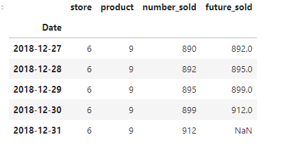

As you can see, the shift operation moved the values number_sold up by 1 position. Let’s calculate the difference between the current number of sold and the future.

# Calculate the difference between current and future number_sold
data['sold_difference'] = data['future_sold'] - data['number_sold']
data.tail()

5. Rolling Windows

A rolling window is a range of selected data for which we intend to apply a function. Functions such as mean, sum, min, and max can be used with .rolling(). For instance, the mean value of number of items sold for every three consecutive days in the dataset goes thus:

# Calculate rolling mean over a window of size 3
data['rolling_mean'] = data['number_sold'].rolling(window=3).mean()

# You decide on a window size, here 3days
data.head()

6. Differencing

Differencing can be used to remove trends from time series data. For example, if your data shows a gradual increase over time, differencing transforms it into a dataset where each value represents the change from the previous value. Let’s find the difference in the number of sold.

# Compute differences
data['differencing'] = data['number_sold'].diff()

7. Handling Missing Values

Missing values are represented as NaN (Not a Number) in Pandas. However, there are methods for handling missing values in a time series DataFrame: Forward or backward filling. ffill() (forward filling) fills missing values with the previous non-null value, and bfill() (backward filling) fills missing values with the next non-null value. Although our dataset is free from missing values. You can check for missing values in the dataset with data.isnull().

# Forward fill missing values
df_forward_filled = df.ffill()

# Backward fill missing values
df_backward_filled = df.bfill()

Visualizing Time Series Data with Pandas

While Pandas doesn’t provide interactive visualization capabilities, it can be used with libraries like Matplotlib and Seaborn for static plots. We can make our time series plot more informative and visually appealing using the line style, color, markers, date formatting, annotations, and more in Matplotlib and Seaborn.

Plotting Time Series

import matplotlib.pyplot as plt
# Plot time series 
datadata['number_sold'].plot()plt.show()

You can only make a few observations of the plot above. Reading more on data visualization libraries like Matplotlib and Seaborn will help you know how to extract insights from a dataset.

You can access the full notebook to the sales figure dataset here.

What’s Next?

Things discussed here are just the tip of the iceberg in time series with Pandas. You can gather further information about time series analysis using Pandas by doing an online search, reading documentation, and playing with some exercises.

Thanks for coming this far!

Stay curious, stay persistent, and enjoy the satisfaction of solving problems.

Happy learning!